Here are pictuers of the frozen regions of random ASMs. (definition at end)
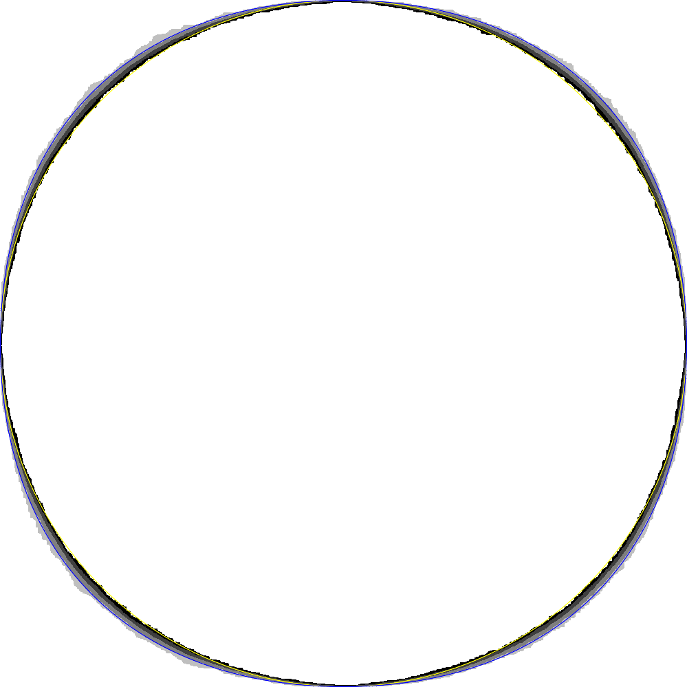
The most interesting pictures are from 100 samples of size 1000 and 10 samples of size 1500 (fixed broken links 7/2012). The pictures use shades of gray to indicate frequency, in my random samples, of the grid points being in the frozen region. The first uses 6 buckets of frequency, with breakpoints 0, 10, 50, 90, and 100%. Overlaid are two curves: a yellow circle and portions of four blue ellipses, which are outside the circle. The circle is the boundary of the frozen region for Aztec diamonds and is not expected to be the frozen region for ASMs, but functions as a kind of null hypothesis. The ellipse was proposed by Filippo Colomo and Andrei Pronko. The ellipse is centered at a corner of ASM and tangent to the midpoints of the two opposite sides. If the sides have length 1, the major axis is root-6 and the minor axis root-2. In coordinates so that the ASM fills the square [0,1]x[0,1], one of the ellipses satisfies (x+y-2)^2+3(x-y)^2=3.
Similar pictures from smaller sizes may be downloaded here. The main thing to know about the filenames is that the first number is the size of the ASMs. The extension png indicates a picture like the ones linked above. There are also postscript files (.eps) in the archive. They print nicely, but I find them a hassle to view on computers. If you do want to view them on a computer and zoom in, it may be useful to use a text editor to change the line ".1 size div setlinewidth" (near the end) to "0 setlinewidth" to make the curves as thin as possible.
I generated the samples using Propp-Wilson coupling from the past (binary backoff), implemented by Matthew Blum and Jason Woolever (v1.6 4/1998). The pseudorandom number generator is R250 by S Kirkpatrick and E Stoll, implemented in C by WL Maier. The postscript code is by Henry Cohn.
Here
is the C code for generating random ASMs
(v1.7 1/2007 by
me,
modifying Blum-Woolever to use more of the bits coming out of R250).
Scripts
for manipulating the output to produce the pictures.
I used ImageMagick's command-line "convert" tool.
Aggregate data
for each size (average height functions and freezing frequencies).
These are text files with names like 700-101-199-height, which is
the sum of the height functions for the 100 samples of size 700 with
seed number 101 to 199. The file with "frozen" instead of "height"
counts for each site the number of those samples in which it was
inside the frozen region.
100 samples of size 1000.
This is 14 megabytes compressed and expands
to half a gig of text files.
All
the samples of all sizes, including the previous link. This is 85M and
expands to 4G of text. It is a tar file made up of one file per
size. Those files are bzip'd tar files. Half of this data (the
files whose names end in f) is redundant, being text files of the
frozen regions, easily reconstructed from the height functions
using the supplied scripts; but it compresses well.
The matrix of an ASM or the grid for the six vertex model is offset from the array of the height function and is smaller by 1. The frozen region makes more sense in these other models, so my picture for size 1000 is a square 999 pixels on a side. Perhaps I should have made the boundary run from 0 to N.